Is Batting Performance Related to Players Position in the MLB?

We would like to discern whether there are real differences between the batting performance of baseball players according to their position: outfielder (OF), infielder (IF), designated hitter (DH), and catcher (C). We will use a data set called mlb_2021, which includes batting records of 336 Major League Baseball (MLB) players from the 2021 season. Every player in this data set has over 200 at-bats recorded to insure that data and analysis was accurate for players that play the majority of the season. Below represented in mlb_2021 are shown in Table 1, and descriptions for each variable are provided. The measure we will use for the player batting performance (the outcome variable) is on-base percentage (OBP). The on-base percentage roughly represents the fraction of the time a player successfully gets on base whether they get walked, hit by a pitch, hits a single, double, triple or home run.

Table 1: A snapshot of 25 observation from the data set

In total there are 12 different variables which includes:

• Player

• Pos = Position

• Age

• AB = At-Bats > 200

• R = How many times they scored

• H = Hits

• 2B = Doubles

• 3B = Triples

• HR = Homerun

• RBI = Runs Batted In

• AVG = Batting Average or H/AB

• OBP = On Base Percentage which is roughly equal to the fraction of times a player gets on base safely.

The player’s positions have been divided into four different groups: catcher (C) , designated hitter (DH), infielder (IF), and outfielder (OF). Since the amount of players playing in these different positions may vary, the table below will show the sample size for each position and their sample mean (On-Base Percentage or OBP).

	C	​DH	IF	OF
​Sample Size	42	9	173	112
Sample Mean	.307	.338	.326	.328

Table 2: Sample Size & Mean of Each Position

When you think of variability amongst on base percentage between all the positions, what comes to mind is that would not be constant since catchers and infielders are considered as defensive specialists while designated hitters and outfielders are typically known to be the best hitters. Below shows Figure 1, which is a side-by-side boxplot for the on base percentage. Notice that the variability appears to be approximately constant across groups; nearly constant variance across groups is an important assumption that must be satisfied before we consider the ANOVA approach.

Figure 1 : Side-by-side Boxplots for OBP vs Position

ANOVA Approach

The method of analysis of variance (ANOVA) in this context focuses on answering one question: is the variability in the sample means so large that it seems unlikely to be from chance alone? This question is different from earlier testing procedures since we will simultaneously consider many groups, and evaluate whether their sample means differ more than we would expect from natural variation. In this case to get ANOVA summary for testing whether the average on-base percentage differs across player position, we use JMP. Below shows the summary of fit and analysis of variance in Table 3.

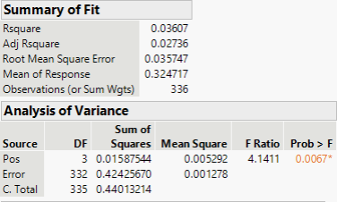
Table 3: Summary of Fit & ANOVA Summary for OBP for Different Position Players

Hypothesis Testing (P-Value Approach)

In this case the null and alternative hypothesis is:

H0: C=DH=IF=OF or the average on-base percentage is equal across the four positions.

HA: The average on-base percentage (i) differ across some (or all) groups.

When conducting the p-value approach we consider what the critical value is = 0.05 and if the p-value is less than the critical value then we reject the null hypothesis, but vice versa if the p-value is greater than the critical value. Looking at Table 3 we have the p-value = 0.0067 which is less than the critical value 0.05. Ultimately we reject the null hypothesis and conclude that the average on-base percentage across some (or all) groups.

Graphical Diagnostics for an ANOVA Analysis

We must check for three conditions when it comes to conducting an ANOVA analysis. First, all observations must be independent, if the data are a simple random sample from less than 5% of the population then this condition is satisfied. Second is the data in each group must be nearly normal, the normality assumption is especially important when the sample size is small. The normal probability plots for each group of the MLB data is shown below, there is some deviation from normality for infielders but this is not a concern since there are about 170 observations in that group without extreme outliers. Third, the variance within each group must be approximately equal, this last assumption is that the variance in the groups is about equal from one group to the next. This can be checked by examining a side-by-side boxplot of the outcomes across the groups like in Figure 1.

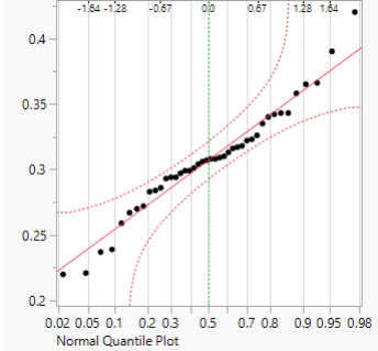
Figure 2: Normal probability plot of OBP for Catchers

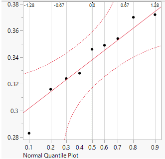
Figure 3: Normal probability plot of OBP for Designated Hitters

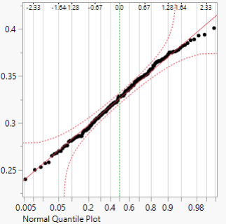
Figure 4: Normal probability plot of OBP for Infielders

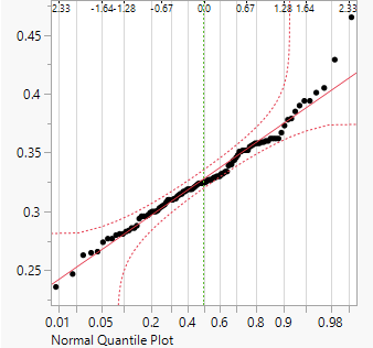
Figure 5: Normal probability plot of OBP for Outfielders

In conclusion, we discovered that essentially hitting performance is somewhat related to player position. It was known in the baseball community that catcher (C) with high AVG or OBP is not common. Surprisingly enough catchers OBP is off from infielders and outfields sample means by close to 20 points or .020. The thing with baseball is that a 0.020 difference in your OBP or AVG could be the difference maker of receiving the MVP award at the end of the season. It is very interesting to see how close infielder and outfielder hitters are in OBP, this shows that hitters performance is evolving into a whole team or lineup effort in results. The ANOVA process shared great results of differentiating hitters that play different fielding positions and this shows that MLB’s idea of making the sport more entertaining by scoring more runs or more action on average will bring more viewership. Ultimately position does matter for hitting performance by the player and this may result as a key factor in close game live decision.