Predicting Home Sales Price in the Midwest (Part 2)

The data contains a sample of 522 observations and 13 variables collected during the year of 2002. This dataset provides information on residential home sales in midwestern cities. The variables that will be specified in this study consist of sales price of residence (in dollars), finished area of residence (in square feet), presence or absence of swimming pool, and presence or absence of air conditioning. The response variable (Y) is the sales price (continuous variable). The explanatory variables are the finished area (X1, continuous variable), presence or absence of swimming pool (X2, dummy; 1 if yes, 0 otherwise), and presence or absence of air conditioning (X3, dummy; 1 if yes, 0 otherwise).

The linear regression model of sales price on the swimming pool dummy only is

Sales Price = 272,396 + 79,724 x pool.

𝛽0 = 272,396: The estimated mean of the sales price of a residence with no pool is $272,396.

𝛽1 = 79,724: The estimated difference in mean sales price comparing residence with a pool and residence without a pool is $ 79,724.

We are testing the hypothesis

Ho: 𝛽1 = 0; H1: 𝛽1 ≠ 0

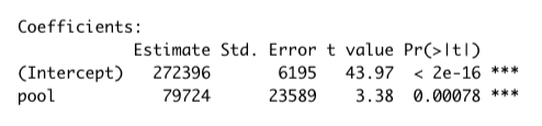
Based on the summary table above the P-value = 0.00078 which is less than the 0.05 significance level. Thus we reject the null hypothesis and conclude that the slope coefficient is statistically significant. This means that there is a significant difference between the mean change in sales price comparing residence with a pool and residence without a pool.

The multiple linear regression model of sales price on swimming pool, area of residence, and their interaction is Sales Price = -88,539 + 161.91 x residence area + 105,909.97 x pool - 37.21 x residence area x pool.

The estimated regression model for residence with a pool is

Sales price = -88,539 + 161.91 x residence area + 105,909.97 x 1 - 37.21 x residence area x 1 = -88,539 + 161.91 x residence area + 105,909.97 - 37.21 x residence area x 1

= (-88,539 + 105,909.97) + (161.91-37.21) x residence area = 17,370.97 + 124.7 x residence area

The estimated regression model for residence without a pool is

Sales price = -88,539 + 161.91 x residence area + 105,909.97 x 0 - 37.21 x residence area x 0 = -88,539 + 161.91 x residence area. Below shows a plot of both regression lines.

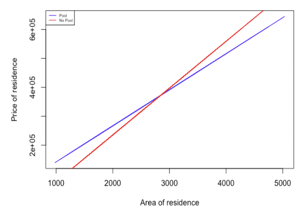
The two lines intersect at a residence area of 2,846.28 square feet and price of $ 372,301.72 as computed below.

Sales price = 17,370.97 + 124.7 x residence area

Sales price = -88,539 + 161.91 x residence area

When we equate the two equations above, we find

17,370.97 + 124.7 x residence area = -88,539 + 161.91 x residence area, where residence area = 2,846.28.

The plot clearly shows that there is an interaction between a residence area with a pool and residence area without a pool. It also shows as the area of residence (with or without a pool) increases, the price of the residence increases.

We are testing the hypothesis

Ho: 𝛽3 = 0; H1: 𝛽3 ≠ 0

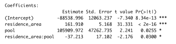
Based on the summary table above the P-value = 0.0300 which is less than the 0.05 significance level. We therefore reject the null hypothesis and conclude that the interaction coefficient is statistically significant. This means that the two regression lines for residence with a pool and residence without a pool are not parallel.

The multiple linear regression model of sales price on swimming pool dummy, AC dummy and their interaction

Sales price = 189,578.2 + 421.8 x pool + 100,875.8 x AC + 65,876.5 x pool x AC.

The estimated mean sale price a residence with no pool and no AC is

Sales price = 189,578.2 + 421.8 x 0 + 100,875.8 x 0 + 65,876.5 x 0 x 0 = $ 189,578.20.

The estimated mean sale price a residence with no pool but with AC is

Sales price = 189,578.2 + 421.8 x 0 + 100,875.8 x 1 + 65,876.5 x 0 x 1 = 189,578.2 + 100,875.8

= $ 290,454.

The estimated mean sale price a residence with pool but no AC is

Sales price = 189,578.2 + 421.8 x 1 + 100,875.8 x 0 + 65,876.5 x 1 x 0 = 189,578.2 + 421.8

= $ 190,000.

Lastly, the estimated mean sale price a residence with pool and AC is

Sale price = 189,578.2 + 421.8 x 1 + 100,875.8 x 1 + 65,876.5 x 1 x 1 = 189,578.2 + 421.8 + 100,875.8 + 65,876.5 = $ 356,752.30.

In conclusion, the presence or absence of a swimming pool and air conditioning system has an effect on the sales price of a residential home in midwestern cities. A home with a swimming pool and an air conditioning system is more expensive than one without any one of those amenities. The data also shows that there is an interaction between the swimming pool and area of residence.