Survey Sampling of the 1980 IPUMS

This dataset focuses on the United States Census Integrated Public Use Microdata Series (IPUMS) from Ruggles, S., Sobek, M., Alexander, T., Fitch, C. A., Goeken, R., Hall,P. K., et al. (2004) . This dataset includes the natural logarithm of Income (Natural Log of Income = ln(Income)), Age, and Gender. This dataset contains a sample size of 500 people meanwhile the population size is 44,846 people. Of that population, 23,533 are male and 21,313 are female. The average age for this population is about 42.4 years old.

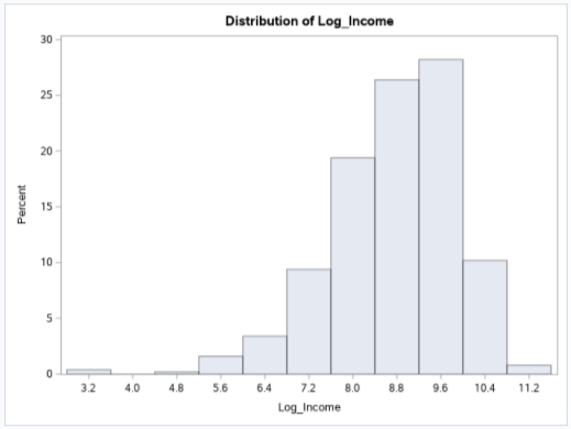
The histogram shows that the majority of people have a log income between 7.6-10 (About 74%). It is expected that only some of the population log income is less than 7.6 and greater than 10.

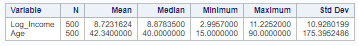
Log Income has a mean of 8.72 and a standard deviation is 10.93 which makes sense since there is a large population in this sample. It is interesting to see the log income mean is a higher percentage of the population when comparing it to the histogram. The sample age has a mean of about 42.34 (similar to what was stated in the introduction) and the standard deviation is 175.39. It is interesting to see how the sample age ranges from 15 years old to 90 years old for its minimum and maximum.

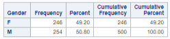
In the sample size of 500 there are 254 males and 246 females. The percentages of males and females are very close to one another.

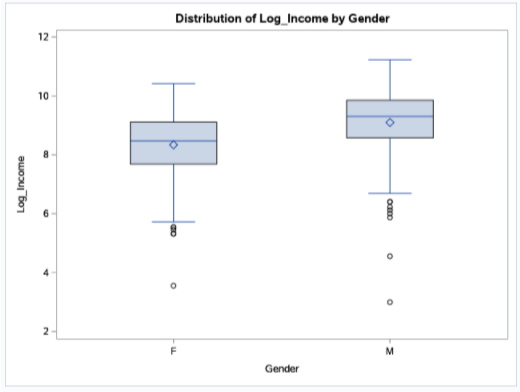
Above is the box plot of log income that identifies male’s have the higher log income with the higher mean (mean is the diamond), but male’s range is more spread out than females. The male’s log income ranges from 7 to about 11.5 (disregarding outliers) and the female’s log income ranges from 5.5 to about 10.5 (disregarding outliers).

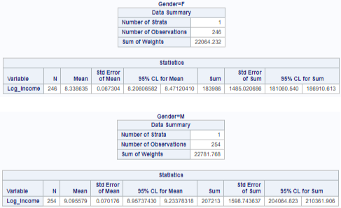
The female’s population mean log income is 8.34 with a standard error of 0.067, and a confidence interval of [8.21, 8.47]. The male’s population mean log income is 9.09 with a standard error of 0.070, and a confidence interval of [8.96, 9.23]. Comparing the population mean log income of male and female, we can conclude that male’s have a higher mean log income by 0.75.

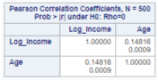
The correlation coefficient between log income and age is 0.148. This is a positive correlation, but this is not a strong correlation between these two variables (A strong correlation is greater than or equal to 0.75).

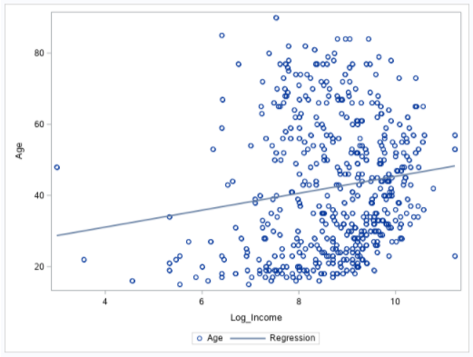
This scatter plot shows a regression line that has a positive correlation, but like the correlation coefficient is not a strong correlation. We can see that there are a large density of points between the 8 to 10 log income range and 18 to 35 age range, which shows this age range makes a fair amount of the log income.

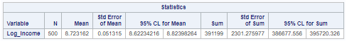
While doing the simple random sampling analysis the population mean of log income is 8.723 and having a standard error of 0.0513. The 95% confidence interval is [8.62, 8.24], which means that estimate is accurate.

While doing the ratio estimation analysis the population mean of log income is 8.735 with a standard error of 0.1701. The 95% confidence interval is [8.40, 9.07], which means that the estimate is accurate but not as accurate is the simple random sampling estimation.

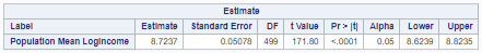
Lastly, the regression estimation analysis of the population mean of log income is 8.723 with a standard error of 0.0508. The 95% confidence interval is [8.62, 8.82], which means that the estimate is the most accurate estimate amongst the three.